pnlf

last updated 2022.01.25

A Python package to analyse MUSE data and measure the Planetary Nebula Luminosity Function (PNLF).

Description

This repository contains the code for Scheuermann et al. (2022).

The data used in this project has been observed for the PHANGS collaboration (Emsellem et al. 2022).

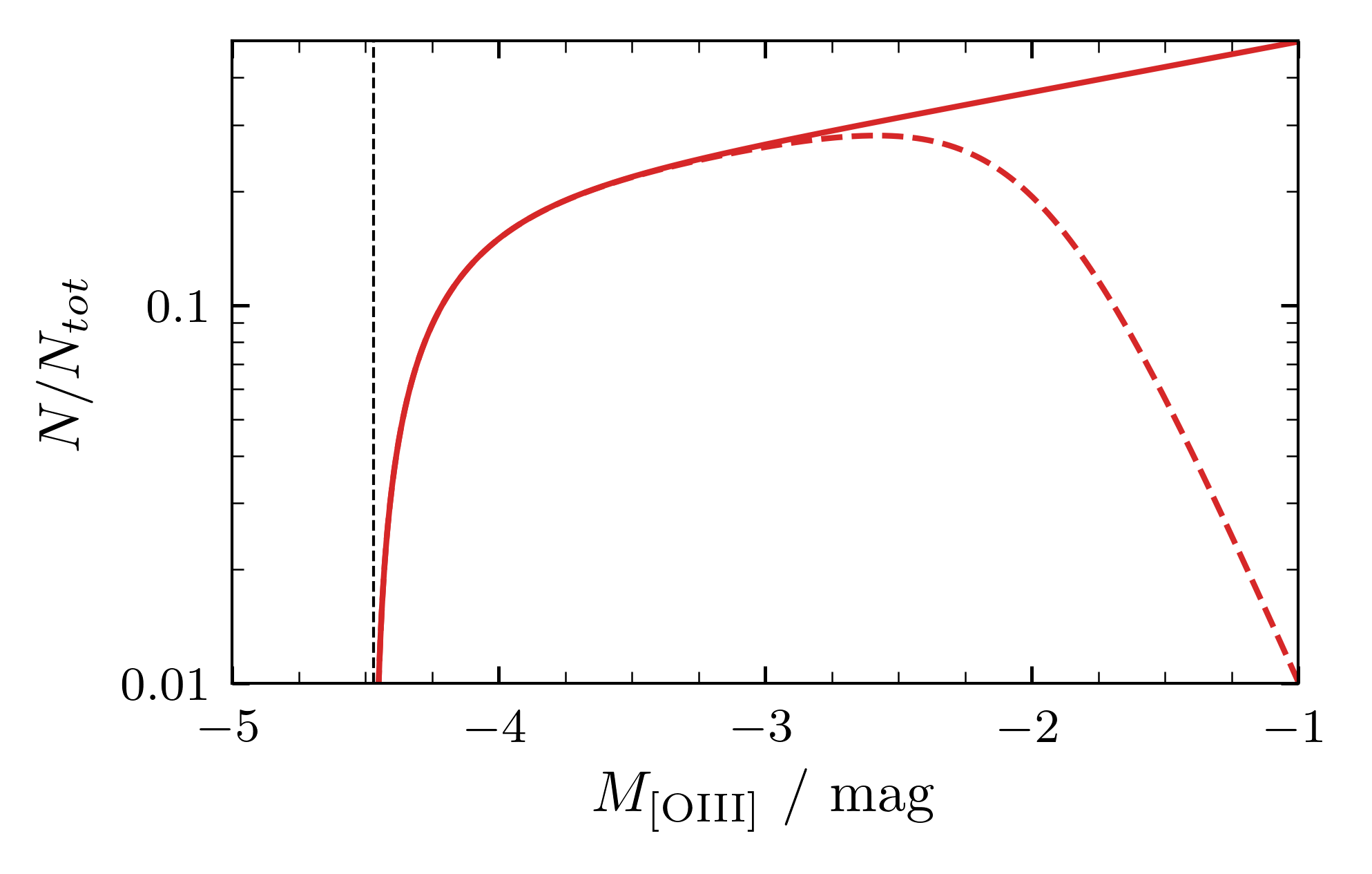
The planetary nebula luminosity function (PNLF) is an empirical relation that can be used to measure the distance to nearby galaxies.

A detailed description of the functionality is either provided by the docstrings of the functions and classes or in the jupyter notebooks. They are annotated with additional background information on what is happening.

Installation

In principle one could clone this repository from github and use it right away. However to ensure that everything works as intended, a few additional steps are recommended.

1. Set up conda environment: It is highly advised to run data science projects in a dedicated environment. This has the advantage that any third party packages have the correct version installed which helps to make the results reproducible. We use conda to do this. The required packages are listed in environment.yml and a new environment, called pymuse is created with

   conda env create -f .\environment.yml

   Every time one opens a new shell, the environment must be activated with

   conda activate pymuse

   New packages can either be installed by altering the installation file and running

   conda env update -f environment.yml --prune

   or by typing

   conda install photutils -c astropy

   Both cases require an active environment. Lastly, a useful addition when working with jupyter notebooks are extensions which can be activated with

   conda install -c conda-forge jupyter_contrib_nbextensions
   conda install -c conda-forge jupyter_nbextensions_configurator

   The extensions can then be activated in the Nbextensions tab of the jupyter explorer

2. Install the package: with the dependencies installed, we still need to setup the actual package. To develop the package, simply type

   python setup.py develop

And that's it. You may have noticed that the project already contains folders and files for unit test and documentations. However neither are currently used but both should eventually be added.

The raw data for the project is supposed to be stores in /data/raw. However since I do not have enough space on my hard drive, I keep those files on an external drive. For easy access I created a symbolic link between the two folders like so

mklink /J data\raw g:\Archive

(see this link for more information on symbolic links)

Project structure

The structure of this project was inspired by this blog post and was set up using PyScaffold 3.2.3. It consists of the following files and folders:

├── AUTHORS.rst             <- List of developers and maintainers.
├── CHANGELOG.rst           <- Changelog to keep track of new features and fixes.
├── config.ini              <- 
├── LICENSE.txt             <- License as chosen on the command-line.
├── README.md               <- The top-level README for developers.
├── data
│   ├── catalogues			<- Final catalogues of objects
│   ├── external            <- Data from third party sources.
│   ├── interim             <- Intermediate data that has been transformed.
│   └── literature distances<- Compilation of literature distances from NED
├── docs                    <- Directory for Sphinx documentation in rst or md.
├── environment.yaml        <- The conda environment file for reproducibility.
├── notebooks               <- Jupyter notebooks. 
├── references              <- Data dictionaries, manuals, and all other materials.
├── reports                 <- Generated analysis as HTML, PDF, LaTeX, etc.
│   ├── catalogues          <- 
│   └── figures             <- Generated plots and figures for reports.
├── scripts                 <- Python script that are used for final run
├── setup.cfg               <- Declarative configuration of your project.
├── setup.py                <- Install for development or create a distribution.
├── src
│   └── pnlf                <- Python package where the main functionality goes.
└── tests                   <- Unit tests which can be run with `py.test`.

Usage

This is an example on how to use this package.

1. Read a fits file from the MUSE data release pipeline (MUSEDAP). This assumes that you have a folder NGC628 inside your raw folder (for more details, see the documentation of ReadLineMaps)

   from pathlib import Path
   from pnlf.io import ReadLineMaps
   
   data_folder = Path('../data/raw')
   NGC628 = ReadLineMaps(data_folder / 'NGC628')

2. Search for point sources in the [OIII] linemap

   from photutils import DAOStarFinder
   from pnlf.detection import detect_unresolved_sources
   
   sources = detect_unresolved_sources(NGC628,['OIII5006'],DAOStarFinder)

3. Measure the fluxes for the previously detected objects

   from pnlf.photometry import measure_flux 
   
   aperture_size = 2.5   # aperture size in fwhm
   power_index = 2.3	  # power index of the moffat (used for aperture correction)
   Ebv = 0.062 		  # galactic foreground extinction for this galaxy
   
   flux = measure_flux(NGC628,
                       sources,
                       alpha=power_index,
                       Rv=3.1,
                       Ebv=Ebv,
                       aperture_size=aperture_size)

4. Emission line diagnostics to classify each object

   from pnlf.analyse import emission_line_diagnostics
   
   mu,mu_err = 29.9, 0.1 		# initial guess for the distance modulus
   completeness_limit = 29		# completeness limit of our data
   
   tbl = emission_line_diagnostics(flux,mu,
                                   completeness_limit,
                                   distance_modulus_err=mu_err) 

5. Fit the PNLF

   from pnlf.analyse import MaximumLikelihood1D, pnlf, cdf
   from pnlf.plot.pnlf import plot_pnlf
   from pnlf.auxiliary import mu_to_parsec
   from scipy.stats import kstest
   
   Mmax = -4.47
   
   
   data = tbl[np.where((tbl['type']=='PN') & (tbl['mOIII']<completeness_limit))]['mOIII']
   err  = tbl[np.where((tbl['type']=='PN') & (tbl['mOIII']<completeness_limit))]['dmOIII']
   
   fitter = MaximumLikelihood1D(pnlf,data,err=err,mhigh=completeness_limit,Mmax=Mmax)
   mu,mu_p,mu_m = fitter([29])
   
   d,(dp,dm)=mu_to_parsec(mu,[mu_p,mu_m])
   print('{:.2f} + {:.2f} - {:.2f}'.format(mu,mu_p,mu_m))
   print('{:.2f} + {:.2f} - {:.2f}'.format(d,dp,dm))
   
   ks,pv = kstest(data,cdf,args=(mu,completeness_limit))
   print(f'statistic={ks:.3f}, pvalue={pv:.3f}')
   
   binsize = (completeness_limit-Mmax-mu) / 5
   
   filename = f'NGC0628_PNLF'
   axes = plot_pnlf(data,mu,completeness_limit,
                    binsize=binsize,mhigh=28.5,
                    Mmax=Mmax,
                    filename=filename)